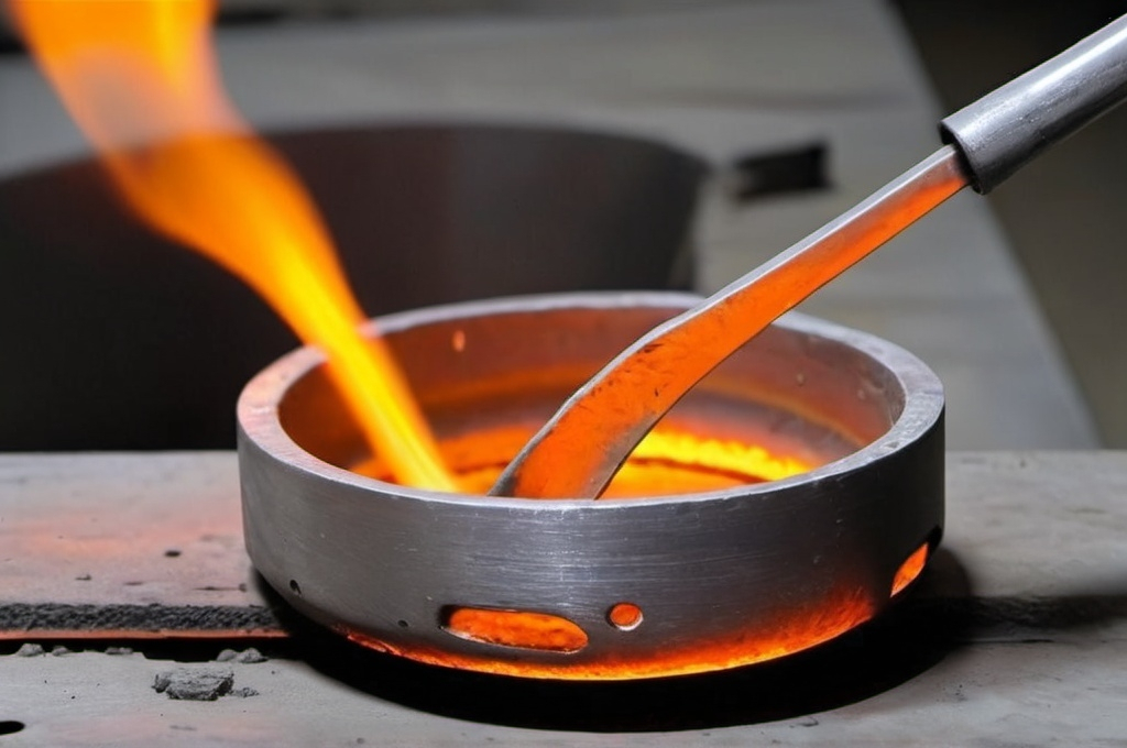
In the realm of optimization algorithms, simulated annealing stands out as an elegant method that draws inspiration from the physical process of annealing in metallurgy. This powerful algorithm has found applications across diverse fields, from logistics to machine learning, offering a unique approach to solving complex optimization problems.
What is Simulated Annealing (SA)?
Origins and Key Concepts of the Simulated Annealing Algorithm
Simulated annealing derives its name and core principles from the metallurgical process of annealing, where metals are heated to high temperatures and then slowly cooled to reduce their defects and increase their strength. Developed in the 1980s by Kirkpatrick, Gelatt, and Vecchi, the algorithm mathematically mimics this physical process to find optimal solutions in complex problem spaces.
The fundamental idea behind simulated annealing is that controlled randomness, much like the random motion of atoms during the cooling process, can help find better solutions to optimization problems. As the temperature decreases, the system gradually settles into a state of minimum energy, which in optimization terms translates to finding a solution that minimizes (or maximizes) the objective function.
Why Use the Simulated Annealing Algorithm for Optimization?
Simulated annealing offers several unique advantages that make it particularly suitable for complex optimization problems. Unlike gradient-based methods that can easily get trapped in local optima, SA’s ability to accept worse solutions probabilistically allows it to explore the solution space more thoroughly. This characteristic makes it especially valuable for problems with many local optima or discontinuous objective functions.
How the Simulated Annealing Algorithm Works
The Concept of Temperature in Optimization
The temperature parameter in simulated annealing controls the algorithm’s exploration-exploitation balance. At high temperatures, the algorithm freely explores the solution space, regularly accepting moves that worsen the current solution. As the temperature decreases according to a cooling schedule, the algorithm becomes increasingly selective, focusing more on exploiting promising regions of the solution space.
The cooling schedule is crucial to the algorithm’s success. Common approaches include linear cooling, where temperature decreases linearly with each iteration; geometric cooling, where temperature is multiplied by a constant factor less than one each time; and adaptive cooling, where temperature adjustment is based on the algorithm’s progress.
Escaping Local Minima with Probabilistic Moves
One of SA’s most distinctive features is its ability to escape local optima through probabilistic acceptance of worse solutions. This acceptance probability is governed by the Metropolis criterion, inspired by principles from statistical mechanics. The probability of accepting a worse solution depends on the magnitude of the solution’s degradation, the current temperature, and the Boltzmann probability distribution.
Real-World Applications of the Simulated Annealing Algorithm
Route Optimization for Logistics
In logistics and supply chain management, simulated annealing has proven highly effective for solving vehicle routing problems. The algorithm can optimize delivery routes considering multiple constraints such as time windows for deliveries, vehicle capacity limitations, driver working hours, and fuel efficiency optimization. Companies implementing SA-based routing systems have reported significant cost reductions and improved delivery efficiency, with some achieving up to 20% reduction in total route distances.
Financial Portfolio Balancing
Financial institutions use simulated annealing to optimize investment portfolios by finding the best asset allocation that maximizes returns while minimizing risk. The algorithm can handle complex constraints such as sector diversification requirements, transaction costs, risk tolerance levels, and minimum and maximum position sizes. This flexibility makes it particularly valuable in real-world financial applications where multiple competing objectives must be balanced.
Machine Learning Hyperparameter Tuning
In machine learning, simulated annealing has become increasingly popular for hyperparameter optimization. The algorithm can efficiently search through the hyperparameter space to find configurations that optimize model performance. This application is particularly valuable because the search space is often non-continuous, objective functions are typically non-differentiable, and multiple local optima exist in the parameter space.
Comparison Between Simulated Annealing and Other Heuristics
Simulated Annealing vs. Genetic Algorithms
While both approaches are inspired by natural processes, they differ significantly in their operation and characteristics. Simulated annealing works with a single solution at a time, using temperature-controlled randomness and generally requiring less memory. It’s often simpler to implement than genetic algorithms, which maintain a population of solutions and use evolutionary operators like crossover and mutation. Genetic algorithms can explore multiple regions simultaneously and may find diverse sets of good solutions, but at the cost of increased complexity and memory requirements.
Simulated Annealing vs. Tabu Search
Tabu Search and Simulated Annealing represent different approaches to escaping local optima. While simulated annealing uses probabilistic acceptance of worse solutions and requires temperature parameter tuning, Tabu Search relies on memory structures to avoid cycling and uses deterministic move acceptance. The memory-less operation of SA contrasts with Tabu Search’s requirement for careful design of tabu lists and aspiration criteria.
Benefits and Drawbacks of the Simulated Annealing Algorithm
Advantages of Using Simulated Annealing
Simulated annealing provides theoretical guarantees of finding the global optimum given infinite time and shows remarkable ability to handle non-continuous and noisy objective functions. Its relatively simple implementation compared to other metaheuristics, combined with flexibility in adapting to different problem types, makes it an attractive choice for many optimization scenarios. The algorithm particularly shines in large-scale optimization problems where traditional methods might fail.
Challenges and Limitations
Despite its strengths, simulated annealing faces certain limitations. Its performance heavily depends on the cooling schedule design, and it may require significant computation time for complex problems. Parameter tuning can be challenging and problem-specific, and there’s no guarantee of finding the global optimum in finite time. The single-solution nature of the algorithm means it might miss alternative good solutions that could be valuable in practice.
In conclusion, simulated annealing represents a powerful and versatile optimization technique that continues to find new applications across various fields. Its unique ability to escape local optima through controlled randomness, combined with its relatively simple implementation, makes it an attractive choice for many optimization problems. While it requires careful parameter tuning and may not always be the fastest option, its reliability and adaptability ensure its place among the most valuable tools in the optimization toolkit.
